From time to time I want to optimize a system, or at least explore how sensitive it is to changes. For example, I may want to optimize (i.e. reduce) the curing time of an epoxy, with the parameters being the curing temperature and the dispensing quantity or method. Or maybe the epoxy is of a two-compound type and I want to find out how critical the mixing ratio is, and whether the process window can be extended by (additional?) temperature curing.

In any of these cases I would want to proceed in a structured manner. Meaning, I would want to pin point the issues quickly and with as few dead ends as possible.

These are situations in which so-called “designed experiments” come to play.

Demonstrating advantage of Factorials vs Changing Factor

There are two different approaches to exploring a parameter space: the one-factor-at-a-time (OFAT) and the factorial approach. As the name suggests, in OFAT you change just and exactly one factor per run of the experiment. The idea is, that if you change too much at the same time, you’ll never know what actually contributed to the observed change. In the factorial approach you’re still worried about confusing results, but you mix them anyway. Yet, the mixing has to happen in a controlled manner: you want to leverage statistics to extract additional gains.

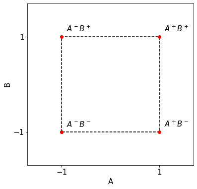
For this discussion to take place, we first need some terminology and definitions. Say we have two parameters $A$ and $B$, and we measure both at a high $A^+$ and a low level $A^-$ (respectively, at $B^+$ and $B^-$).

For example, we could investigate the curing behavior of a certain epoxy. In this, parameter $A$ could be the curing temperature, and $B$ the dispensing method. Assume a high $A^+$ of $80\,°C$ and a low level at room temperature, or $20\,°C$. Assume further there to be two dispensing methods: $B^+$, which applies the epoxy quantity as two layers, with a second layer applied 2h after having dispensed the first. $B^-$ is applying the full quantity in one go. The curing of the epoxy is determined after 4h curing time by means of a test. Such a test could be a shear test to probe the mechanical strength, or an electrical resistance measurement, etc. depending on the task at hand.

The ground truth relation between the two parameters is
$$
\begin{align}
y(x_A, x_B) = \beta_0 + \beta_Ax_A + \beta_Bx_B + \varepsilon
\label{eq:two_factor_model}
\end{align}
$$
With the example from above, $y$ is the progress in epoxy curing after said set curing time. It is a function of the temperature $x_A$ (in our case we’re only looking at the two points $x_a=\{A^-,\,A^+\}$), and the dispensing method $x_B$ (again evaluated only at $x_b=\{B^-,\,B^+\}$). For the moment, with this function we assume that the two parameters do not interact with each other (there is no factor $x_Ax_B$). The ground truth has a certain offset $\beta_0$. The factors $\beta_A$ and $\beta_B$ describe how sensitive $y$ reacts to changes in $x_A$ and $x_B$, respectively.And finally, the factor $\varepsilon$ accounts for random error.

Note, the ground truth is what the universe has in stores for whatever is going on. By making an experiment, we evaluate this function (meaning, we measure $y$) at discrete points (meaning, given $x_A$ and $x_B$). Once we have conducted enough experiments, we can reconstruct an estimate of the ground truth. This reconstructed ground truth then allows us to make future predictions as of how the system will behave given different values of input parameters $x_A$ and $x_B$. Yet, while the universe is unfailable, we — the experimenters — are. Meaning, there will be measurement errors. For one, the model already accounts for $\varepsilon$. Additionally, if we apply a certain $x_i$ in two different runs of the experiment, there will also be an uncertainty about the exact level and value that was actually applied.

For simplicity we assume the random error to scale with $\beta_0$, namely for $\varepsilon$ to be Gaussian distributed around zero with variance $\beta_0$ (i.e. standard deviation $\sqrt{\beta_0}$):
$$
\varepsilon(z) = \frac{1}{\sqrt{2\pi\beta_0}} \mathrm{exp}(\frac{z^2}{2\beta_0}).
$$

Changing Factor (OFAT)

In a one-factor-at-a-time (OFAT) approach, we keep $B$ at the low level $B-$ and vary $A$ to the low and high level; and vice versa. To estimate the effect of a changing factor $A$ we can look at the difference $A^+-A^-$. Respectively, written with $B^-$ taken into account: $\beta_A’ = \frac12(A^+B^–A^-B^-)$. The $\frac12$ factor is necessary for normalization. Equally, to estimate the effect of a changing factor $B$ we look at $\beta_B’=\frac12(B^+A^–B^-A^-)$.

Note, we’re trying to estimate the ground truth factors $\beta_\cdot$, we’re not pretending to directly measure the ground truth. Hence, we denote the estimators as $\beta_\cdot’$.

In a one-factor-at-a-time approach, we thus have to measure three quantities: $A^+B^-$, $A^-B^+$, and $A^-B^-$. Given the likely presence of measurement error ($|\varepsilon|>0$ in the ground truth function ($\ref{eq:two_factor_model}$)), we’d want to repeat the measurement of the three quantities $N$ times. The total number of measurements taken in a one-factor-at-a-time approach is thus $M = N\times3$.

To judge the efficiency of the estimations of $\beta_\cdot’$ we can look at the estimation error $\Delta_\cdot$. The estimation error refers to the difference in estimated $\beta_\cdot’$ to the ground truth $\beta_\cdot$. The estimation $\beta_\cdot’=\beta_\cdot'(N)$ is a function of the number of measurements $N$ the quantities $A^+B^-$, $A^-B^+$, and $A^-B^-$ were averaged over. To filter the variability in random error $\varepsilon$ in ($\ref{eq:two_factor_model}$), we average the estimation error over $n_\mathrm{comp}$ comparison estimates:
$$
\begin{align}
\Delta_\cdot(n_\mathrm{comp}, N) = \frac{1}{n_\mathrm{comp}}\sum_i^{n_\mathrm{comp}}|\beta_{\cdot,i}'(N)-\beta_\cdot|.
\label{eq:diff_estim}
\end{align}
$$

Factorial

In a factorial approach we add a fourth quantity, $A^+B^+$. With this additional quantity we obtain two estimates for $\beta_A$ and $\beta_B$. Or, respectively, we can estimate $\beta_A$ and $\beta_B$ taking the average of those two intermediate estimates.
$$
\begin{align*}
\beta_{A,1}’&=\frac12( (A^+B^–A^-B^-) ) \\
\beta_{A,2}’&=\frac12( (A^+B^+-A^-B^+) )
\end{align*}
$$
$$
\begin{align}
\Rightarrow\quad \beta_A’&= \frac12(\beta_{A,1}’ + \beta_{A,2}’) = \frac14(A^+B^+ + A^+B^- – A^-B^+ – A^-B-)
\label{eq:diff_estim_fact_A}\\
\Rightarrow\quad \beta_B’&=\frac14(A^+B^+ + A^-B^+ – A^+B^- – A^-B-)
\label{eq:diff_estim_fact_B}
\end{align}
$$

Efficiency in estimators

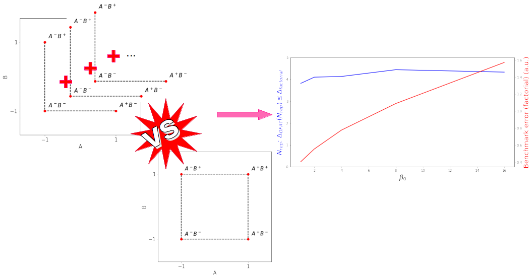
We can again observe the efficiency of the estimators ($\ref{eq:diff_estim_fact_A}$) and ($\ref{eq:diff_estim_fact_B}$) over $n_\mathrm{comp}$ comparison estimates through ($\ref{eq:diff_estim}$). Furthermore we’d like to compare the efficiency of the estimators of the one-factor-at-a-time with the factorial approach. The only difference in the two approaches is that there is the additional quantity $A^+B^+$ in the factorial approach. Consequentially, if $N=1$, the one-factor-at-a-time approach has to conduct only 3 measurements, whereas the factorial approach requires 4 measurements. Yet, for $N=2$, the one-factor-at-a-time approach is already at 6 measurements, and so on.

By keeping the factorial approach limited to the minimally required 4 measurements, we’d like to see how large $N$ has to be for the one-factor-at-a-time error ($\ref{eq:diff_estim}$) to be equal or lower to the factorial estimator error.

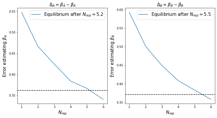
Superior efficiency of factorial approach

The estimation factor of the one-factor-a-time (OFAT) approach, $\Delta_\mathrm{OFAT}$, starts off large and decreases with $n_\mathrm{comp}$ as expected. Nonetheless, to obtain an error of equal size to the factorial approach, the OFAT approach has to average over about $N_\mathrm{rep}=4$ repeated measurements. This means, while the factorial approach works with 4 measurements to be taken, an equivalent OFAT approach requires $M=3\times N_\mathrm{rep}=12$ measurements.

But surely, for more noisy experiments, the OFAT approach and the inherent $N_\mathrm{rep}>1$ reproduction of the different measurements will be supperior to the single reproduced factorial approach?

The answer is “no”: While the error does increase for both approaches, it increases the same way, which leaves the factorial approach in a lead. So much so in fact, that we can use the factorial estimate as a benchmark and check how many repeated OFAT measurements one needs on average to get the error below that of the factorial approach.

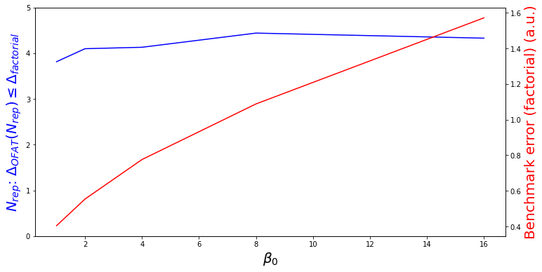
That being said, to generate the above figure I’ve made a few simplifications. Namely, I’ve assumed that $\beta_0=\beta_A=\beta_B$. Maybe if we let $\beta_0$ grow in magnitude, this added noise will be better managed by the OFAT averaging than the one-shot factorial? Well, still “no”.

Conclusion

This post is only an introduction to the topic of designed experiments. More post will follow (click on the “designed experiments” tag to find related posts). But one lesson that you can already take home is this: measure/evaluate the $A^+B^+$ setting! It provides more insights than repeated measurements and subsequent averaging of the other three points in parameter space.

Quantitatively speaking, independent of the magnitude of $\beta_0$ (and thus the amplitude in noise $\varepsilon$), the one-factor-a-time (OFAT) approach requires between 3-4 reproductions (i.e. 9-12 measurements) to be equally efficient as the 4 measurements overall of the factorial approach! In other words, the factorial approach in a two-factor model is about 2-3 times more efficient than the OFAT approach.

Further reading

D.C. Montgomery, ”Design and Analysis of Experiments,” John Wiley & Sons, 8th ed, ISBN 978-1118-14692-7