The “one factor at a time (OFAT)” approach isn’t suited if there is an interaction factor present in a multi factor experiment. In the present post I explore the shortcomings of the OFAT versus factorial approach in more detail.
In a first post about Designed Experiments, I have shown the superior efficiency of a “factorial” approach compared to a “one factor at a time (OFAT)” scheme in a two factor experiment. As it was an introduction to the topic, I left the ground truth function void of any interaction term (i.e. there is no multiplicative $x_Ax_B$). Now, if the two parameters do interact, it should be clear that the OFAT approach cannot converge to an accurate result: the OFAT approach intentionally ignores any interaction, to keep the analysis “clean”. In the present post I thus look closer at the shortcomings of the OFAT — respectively, the superiority of the factorial — approach.
Note, this should be obvious from the introduction to this post thus far, but: I’m going to lean heavily on the terminology introduced in that other post, so please have a look at that one first before continuing reading here.
Efficiency under interaction
The one-factor-a-time (OFAT) approach requires between 3-4 reproductions to be equally efficient (i.e. getting down to the same residual error) as the single measurements of the factorial approach. In the OFAT, 3-4 reproduction mean about 9-12 measurements. In other words, the factorial approach in a two-factor model is about 2-3 times more efficient than the OFAT approach. And this is true independent of the magnitude of $\beta_0$ (and thus the amplitude in noise $\varepsilon$).
In the present analysis I modify the previous two factor model and include an interaction term $\beta_{AB}$.
$$
\begin{align}
y(x_A, x_B) = \beta_0 + \beta_Ax_A + \beta_Bx_B + \beta_{AB}x_Ax_B + \varepsilon
\label{eq:two_factor_interaction_model}
\end{align}
$$
While the OFAT approach was less efficient, under the assumption of $\beta_{AB}=0$, the estimated $\beta_A$ and $\beta_B$ did converge to the estimations of the factorial approach. One had to just consider a relatively large number of replicate measurements $N$.
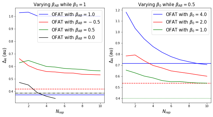
Now, with $\beta_{AB}\neq0$, even by averaging over many $N$, the OFAT is far off the factorial approach. To illustrate this, I calculate four scenarios: while keeping $\beta_0=1$ I vary $\beta_{AB}={0,-0.5,0.5,1}$. Obviously, with $\beta_{AB}=0$ we’re back in the non-interacting scenario; I include it here as reference. It should also be clear that the results with $\beta_{AB}=\pm0.5$ yield the same results, only the magnitude $|\beta_{AB}|$ is relevant.
Additionally, I look at what happens if we increase the relative importance of $\beta_0$ compared to $\beta_{AB}$. Kind of unsurprisingly, the more ground-level noise there is in the system, the less efficient is also the factorial approach given only ONE measurement. And thus the OFAT approach will converge relatively soon to the same residual error as the factorial approach.
However, keep in mind, we’re only comparing factorial with OFAT. The inherent results could both still be plain garbage. In other words, while ONE factorial measurement may be closer to the ground truth value than averaging over many OFAT measurements, the residual error could still be so large that the result from ONE factorial measurement is still not useful. Obviously, in a measurement setup one should be concerned about making an as clean (\beta_0$ small) measurement as possible. Making the setup noisier (enlarging $\beta_0$) won’t improve the measurement.
Put like this, it is not surprising that OFAT approaches the factorial efficiency if $\beta_0/\beta_{AB}\gg1$. It’s just that both results tend towards utter uselessness. The accuracy of the factorial approach will be topic of another post.
Visualization
To visualize the above claims, first I again initiate the same functions as in the previous post.
In the plots below, the solid lines correspond to the residual error ($\Delta_\cdot$) from the ground truth. The horizontal line of corresponding color indicates the (on average, i.e. expected) residual error obtained from ONE factorial experiment. The point at which the two curves intersect shows how many reproductions $N$ the OFAT approach would have to conduct in order to obtain the same efficiency as the ONE factorial experiment. As expected, the OFAT with $\beta_{AB}=0$ (left) converges quickly (i.e. after about 3-4 reproductions) to the factorial benchmark value. On the other hand, the larger $|\beta_{AB}|>0$ gets, the longer it takes for $\Delta_A$ to converge. I actually cut off the plot at $N=10$, the trend should already be rather self-explanatory.
Note that, as mentioned above, the results with $\beta_{AB}=\pm0.5$ yield the same results, only the magnitude $|\beta_{AB}|$ is relevant.
The right sub-plot illustrates that $\beta_{AB}>0$ is less relevant if there is large noise in the system, i.e. $\beta_0\gg0$. But then again, if there is large noise in the system, one ought to improve on the measurement conditions, and/or one must average also over several results obtained with the factorial approach.