Let’s say we conduct a fail/pass test. We subject $n_\mathrm{s}$ samples to an accelerated (representative) life test of $m=1$ lifetime equivalents. The test is considered a success if $100\,\%$ of the $n_\mathrm{s}$ samples survive. Yet, this leaves the important question of how certain can we be that the population as a whole (from which the $n_\mathrm{s}$ samples are a representative sub-set) will survive the $m=1$ lifetime equivalents? And, apart from the implied confidence level, what fraction of the population is still expected to fail even if $100\,\%$ of the $n_\mathrm{s}$ samples did survive?

We consider a binomial distribution: the samples either survive (pass), or die (fail). Each sample has a probability $p$ of dying. Hence, starting with $n_\mathrm{s}$ samples, the probability of ending up with $k$ dead (failed) samples is

$$
B(k) = \frac{n_\mathrm{s}!}{k!(n_\mathrm{s}-k)!} p^k (1-p)^{(n_\mathrm{s}-k)}.
$$

The case of interest is with $k=0$ dead samples at the end of the test, i.e. all passed. This leaves us with the special case of

\begin{equation}
B(0) = (1-p)^{n_\mathrm{s}}.
\label{eq:B0}
\end{equation}

With $p$ being the probability of dying, $(1-p)=R$ can be said to be a measure of the reliability (in the sense of the probability to survive the foreseen lifetime) of the devices being tested. The probability $B(0)$ represents a measure of how often we expect to see this survival rate. In other words, it is $B(0)=(1-C)$, with $C$ the confidence level.

In other words, we can rewrite Eq. (\ref{eq:B0}) as
\begin{equation}
(1-C) = R^{n_\mathrm{s}}.
\label{eq:CRn}
\end{equation}

And from Eq. (\ref{eq:CRn}) follows how $n_\mathrm{s}$ relates to $R$ and $C$:

\begin{equation}
n_\mathrm{s} = \frac{\ln(1-C)}{\ln(R)}.
\label{eq:n_lnCR}
\end{equation}

As a numerical example, let’s assume we want to be $C=90\%$ confident that the whole population shows a $R=90\%$ reliability (i.e. at least $90\%$ of the whole will survive). In this case, the minimum number of samples to test is $n_s = 21.85$, i.e. 22 samples.

Another example is that with $n_s=77$ and an assumed reliability of $R=95.0%$, the confidence level is $C = 98.07%$. Meaning, if we test 77 samples, we should find at least one defective sample in 98% of the cases, if the underlying reliability is less than 95%.

We can reuse already tested samples and expose them to the accelerated life test a second, third, … , $m$ time. Up to a certain point this would be equivalent a higher number of samples. Written differently,

$$
n_\mathrm{s} = m \times n_\mathrm{actual\_samples},
$$

and thus

$$
n_\mathrm{s} = \frac{\ln(1-C)}{m \ln(R)}.
$$

Sidenote, it should be clear that a test conducted with only one sample but which was exposed to $m=100$ lifetimes would NOT be statistically equally meaningful as a test with $100$ samples exposed to $m=1$ lifetime. In what context $m>1$ might be meaningful depends on various circumstances.

The confidence level $C$ is a critical parameter of a fail/pass test. The purpose of a fail/pass test is to learn something (that’s the purpose of any test, of course, not only fail/pass). Often this tool comes into play to confirm that a new product can be launched. However, testing costs money (for the samples) and time (for the actual testing). Hence, small sample sizes are typically preferred.

Yet, confirmation bias aside, what can we possibly learn from a passed test with few samples? Let me assume an extreme case example: testing two samples, which are so inherently flawed that they fail half of the time. Such a test will fail in $C=75\,\%$ of the time. Upon failure the development team would likely investigate the failed sample and subsequently improve it. This could be considered a good outcome.
On the other hand, starting off with an only $R=50\,\%$ reliable product left a lot of room for improvement.

And maybe even worse, there are still $B(0)=25\,\%$ of the time in which the two samples do NOT fail, $25\,\%$ of the time in which the team would not investigate the failure mechanisms, and $25\,\%$ of the time in which the product launch would continue according to schedule and being shipped. It should be without saying, no customer is interested in a $R=50\,\%$ reliable product.

If the product was slightly more reliable (say, a still rather bad $R=70\,\%$), the two samples would pass in $B(0)=49\,\%$ of the cases. In other words, the fail/pass test would be only just slightly more informative than an independent coin-flip!

Numerical examples

Let’s add some images to the discussion.

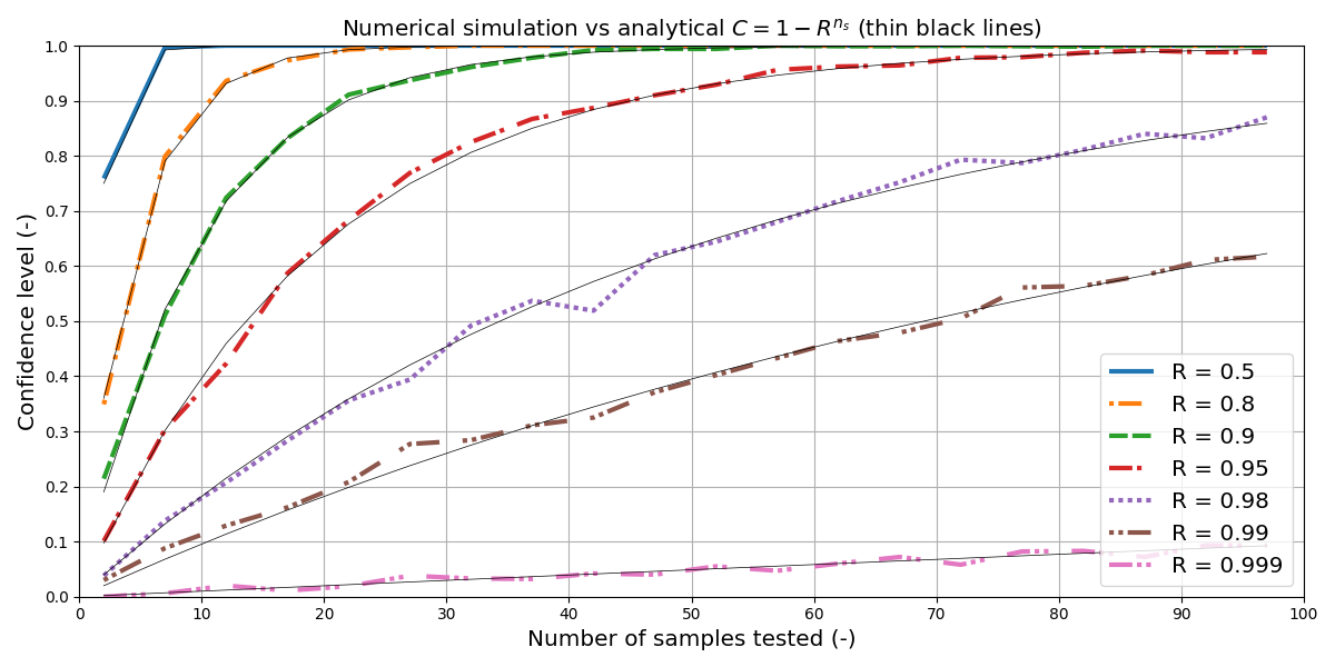
Given $n_\mathrm{s}$ samples which each have an (assumed) intrinsic reliability $R$, how often would we run a test without any sample failing? This rate of at least one failure represents our confidence level that we would have encountered at least one failing sample if the underlying reliability was lower than the assumed $R$.

In the following, I’m going to work with python. I encourage anyone reading this post to copy, execute, and modify the code blocks below to reproduce my images: play around with some of the parameters, get to an understanding where what comes from; that’s the best way to make sense of random processes.

First, I set the stage by defining a basic class called Device. The objects of this class represent the devices under test (DUT). I assume the population of DUTs have a reliability $R$, intrinsic to the population. Some of the DUTs will fail the test, the others will pass it. Which DUT fails is random (after closer inspection one might find that the failing DUTs happen to be unlucky in how the the individual manufacturing tolerances accumulated, for example), and the frequency is given by said intrinsic reliability. Numerically speaking, we take a random value between 0 and 1 and compare it with the set intrinsic reliability. The test() function returns the binary value 1 if the DUT survived the test, 0 if it failed. Note, we’re looking at pass/fail tests: we don’t care how catastrophically the DUT failed the test, we only care whether it did pass or not.

In a test plan we have multiple DUTs (assume $n$) to work with, numbered as $\mathrm{DUT}_0,\ldots,\mathrm{DUT}_{n-1}$. For simplicity, I call the aggregate of these DUTs a test battery. Concretely, by conducting a test, we expose these $n$ DUTs of the test battery to certain conditions (such as temperature shocks, high/low temperature storage, etc.) and then check each individually, whether it is still within the agreed upon specifications — in short, whether it is still alive.

Below a list of parameters I want to explore and visualize.

As a first inspection, we find back the analytical values from above:

• an intrinsic reliability of $R=0.9$, paired with $n_s=22$ samples, gives us a value for the confidence of $C=0.9$ (print_summary(0.9, 22)),
• and with $R=0.95$ and $n_s=77$ samples, we find back the $C=0.98$ (print_summary(0.95, 77)).

All the usual disclaimers regarding statistical explorations apply: The “tested” samples are assumed to be identical and independent. The analytical solution is true only in the limit of infinite repetitions. And so on.

Mapping out R vs C analytically

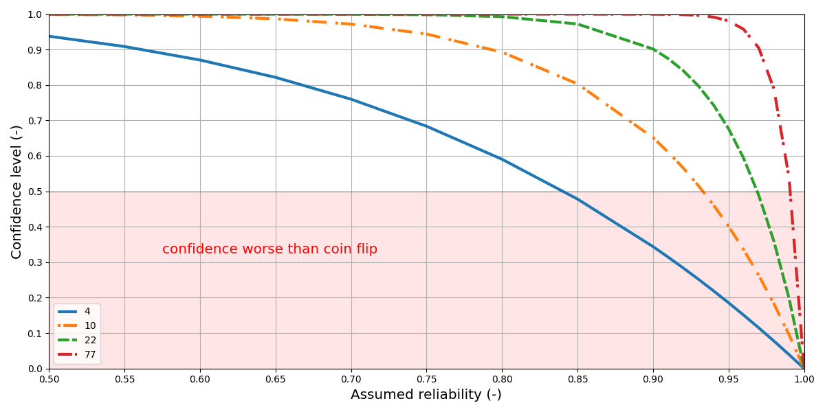
In the above sections we have looked at the question: “how many samples are we supposed to test assuming a target $R$ and $C$?” In the present section we approach the problem from the other side. Assuming we have $n_\mathrm{s}$ samples available, what can we learn from a fail/pass test?

As already mentioned above, if all $n_\mathrm{s}$ samples pass the test, we forego the opportunity to actually learn something (meaning, by opening up a failing sample and learning about the root causes). The only statement we can make given a $100\,\%$ pass rate is that the underlying population is $R$ reliable with $C$ confidence, related to each other through Eq. (\ref{eq:CRn}) and (\ref{eq:n_lnCR}), respectively.

As an example let’s assume we have $n_\mathrm{s}=4$ samples available. What is the underlying reliability $R$ of the population supposed to be for us to have a reasonable chance of catching a failing sample among these $n_\mathrm{s}=4$ samples?

One way to go about answering this question is to flip a coin: tail means the population is impecable and can be shipped, head means the population shows some not-further-specified flaws. This strategy, stated in this extreme form, does not take the fail/pass test into account in any way whatsoever. However, an unrelated coin flip is not actually worth less than a test with expected frequency of finding a failing part of $C\leq0.5$.

For example, if none of the $n_\mathrm{s}=4$ samples failed, but, if at the same time we were to expect the underlying population to show a reliability of at least $R\geq0.84$, then the fact that all $n_\mathrm{s}=4$ samples have passed is actually less informative than a completely unrelated coin flip!

More generally, from Eq. (\ref{eq:CRn}) we find

\begin{equation}
R = \sqrt[\leftroot{-2}\uproot{2}n_\mathrm{s}]{1-C}.
\label{eq:nrootC}
\end{equation}

For a test with $n_\mathrm{s}=4$ to be meaningful — say $C\geq0.9$ — the underlying population has to show a reliability of at most $R=0.56$.

Further reading

This notebook was originally inspired by an Accendo Reliability podcast on the topic, https://accendoreliability.com/podcast/arw/making-use-reliability-statistics/

Regarding what we can learn from a failed vs passed test (equally applicable for software and hardware), recommended
K. Henney “A Test of Knowledge” https://medium.com/@kevlinhenney/a-test-of-knowledge-78f4688dc9cb