The signal to noise ratio (SNR) in a measurement generally improves as one increases the acquisition time, or as one adds up over an increasing number of individual measurements, respectively. The scaling behavior is approximately proportional to the square root of the number of individual measurements.
In this post I derive the argument where this square root scaling behavior comes from.
Definitions
For the following discussion I assume to have a statistical process at hand, whose probability distribution is given by function $f(x)$. A probability distribution is defined such that the total has probability 1 (with 100% certainty every possibility is considered)
$$\int f(x) \mathrm{d}x = 1.$$
Such a distribution has a certain expectation value $\mathrm{E}[x]$, and a variance $\mathrm{V}[x]$. These are defined as
$$\begin{split}
\mathrm{E}[x] :&= \int xf(x)\mathrm{d}x = \mu \quad\small\text{(note: $\mathrm{E}[1]=1$)} \\
\mathrm{V}[x] :&= \int (x-\mu)^2 f(x)\mathrm{d}x = \mathrm{E}[(x-\mu)^2] \\
&= \mathrm{E}[x^2-2x\mu+\mu^2] \quad\small\text{($\mu$ is a number; which we can pull out of the integral)} \\
&= \mathrm{E}[x^2] -2\mu\mathrm{E}[x] + \mu^2\mathrm{E}[1] \\
&= \mathrm{E}[x^2] – 2\mu^2 +\mu^2 = \mathrm{E}[x^2] – \mu^2 \\
&= \mathrm{E}[x^2] – \mathrm{E}[x]^2.
\end{split}$$
The “expectation value” $\mathrm{E}[x]$ is also known as the average value. The “variance” $\mathrm{V}[x]$ is sometimes better known as the “standard deviation” $\sigma$, whereby $\sigma := \sqrt{\mathrm{V}[x]}$.
Signal and noise dynamics
Signal
I assume to conduct a measurement during which I record data. The measured data in the $j$-th measurement $M_j$ I represent using the symbol $D_j$. These data contain (per $j$-th measurement) the real signal $S_j$, but are polluted by some noise $N_j$:
$$D_j = S_j+N_j.$$
During an initial measurement $M_0$ I obtain $D_0$. Over subsequently repeated measurements I add additional data.
$$M_1 = D_0 + S_1 + N_1 = (S_0+S_1) + (N_0+N_1).$$
Let’s go for $n$ measurements. The summed end result is going to be
$$M_n = M_{n-1} + S_n + N_n = \sum_{i=0}^n S_i + \sum_{i=0}^n N_i.$$
The real signal was present in every single measurement, $S_0=S_1=\ldots=S_n=S$.
Therefore, the sum of the signal terms is simply proportional to the number of measurements that we have conducted:
$$\sum_{i=0}^n S_i = \mathrm{E}[S] = nS.$$
Noise
On the other hand, the noise we have to treat differently. To simplify the discussion, I assume the noise is equally distributed around zero (for a more general approach see below). This means, on average negative contributions cancel positive contributions:
$$\mathrm{E}[N] = \int xN(x)\mathrm{d}x = 0.$$
For the noise contribution we’re not interested in the average increase (as per the example, noise around zero cancels out).
In order to treat the growth in noise we have to consider its variance, or its standard deviation, respectively. First, because of the above simplified assumption to be distributed around zero, I rewrite the variance as
$$\mathrm{V}[N] = \mathrm{E}[N^2] – (\mathrm{E}[N])^2 = \mathrm{E}[N^2].$$
The sum of the variances of $N_i$ and $N_j$ is
$$\begin{split}
\mathrm{V}[N_i + N_j] &= \mathrm{E}[(N_i+N_j)^2] – \mathrm{E}[N_i+N_j]^2 \quad (\small\text{simplify: }\mathrm{E}[N]=0) \\
&= \mathrm{E}[N_i^2+2 N_i N_j + N_j^2] = \mathrm{E}[N_i^2] + 2\mathrm{E}[N_i N_j] + \mathrm{E}[N_j^2].
\end{split}$$
I assume random noise that is uncorrelated with itself. With this assumption I cancel the middle term: $\mathrm{E}[N_i N_j]=0$ (essentially, that’s the definition of “uncorrelated”). At the same time, $N_i$ and $N_j$ are from the same noise source. This means, on average, we have $\mathrm{E}[N_i^2] = \mathrm{E}[N_j^2] = \mathrm{E}[N^2]$.
I end up with an expression
$$\begin{split}
\mathrm{V}[N_i + N_j] &= 2\mathrm{E}[N^2] = 2\mathrm{V}[N] \\
\sigma_{i+j} &= \sqrt{2\mathrm{E}[N^2]} = \sqrt{2}\sigma_N.
\end{split}$$
The above argument can be repeated for all $n$ repetitions and thus end up with a summed noise standard deviation
$$\sigma_{1+\ldots+n} = \sqrt{n}\sigma_N.$$
Conclusion
The signal grows linearly with the number of repetitions; $S_{1+\ldots+n} = nS$. On the other hand, noise grows with the standard deviation, and as such only with the square root; $\sigma_{1+\ldots+n} = \sqrt{n}\sigma_N$. As a consequence,
the signal to noise ratio (SNR) improves with $\sqrt{n}$:
$$SNR = \frac{nS}{\sqrt{n}\sigma_N} = \sqrt{n}\frac{S}{\sigma_N}.$$
In the above calculations I have simplified with the assumption $\mathrm{E}[N]=0$. If the noise is not distributed around zero, we can redefine noise as
$$N’ = N – \mathrm{E}[N],$$
which then is distributed around zero. The statistical dynamic still holds. Noise can be Gaussian, or Uniform, or something-else distributed. The above calculation didn’t assume a particularity of one of these distributions.
If the noise is not symmetrically distributed around its average value, then the above calculations don’t work. Nonetheless, the general tendency — for the noise to grow slower than the signal — persists.
Further reading
Check out the Wikipedia entry on Signal averaging.


