As discussed in another post, the signal to noise ratio (SNR) in a measurement generally improves proportional to the square root of the number of individual measurements.

While I have motivated and derived the square root argument heuristically in this other post, in the present one I want to add some images. To generate these images I’m going to work with python. Below I comment code blocks which anyone can copy, execute, and modify to reproduce my images. In fact, I encourage anyone reading this to indeed reproduce the images and play around with some of the parameters: that’s the best way — in my opinion — to make sense of random processes (thus this post in the first place).

Aligning on basic concepts

First, I want to lay down a concept of a “signal”, as well as “noise”. I’m going to work in an arbitrary parameter space, meaning the x- and y-axes of any plots are of arbitrary units. Nonetheless, to have something to work with I choose to set up a number line between 0 and 100 (again, this scale is arbitrary, I just feel good about these round numbers…), which will be the basis for any simulation. And because I lack imagination, I call this number line xx.

Furthermore, to have something non-trivial — say, “interesting” — to work with as the “signal”, I choose a Gaussian function, which I call gauss.

Following the discussion from the SNR post, I will want to simulate the adding up of random noise. To do so, I need a convenient way to generate new noise. The following noise function hands me new noise with an amplitude between 0-1 (of arbitrary units) for every point in xx, whenever it’s called.

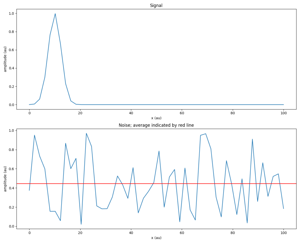
For example, let’s say the underlying ground truth signal is a Gaussian centered around 10 and with a standard deviation of 2.5. Visually, such signal and noise look as follows (the red line inside the noise plot represents the average noise level).

Demonstrating noise canceling

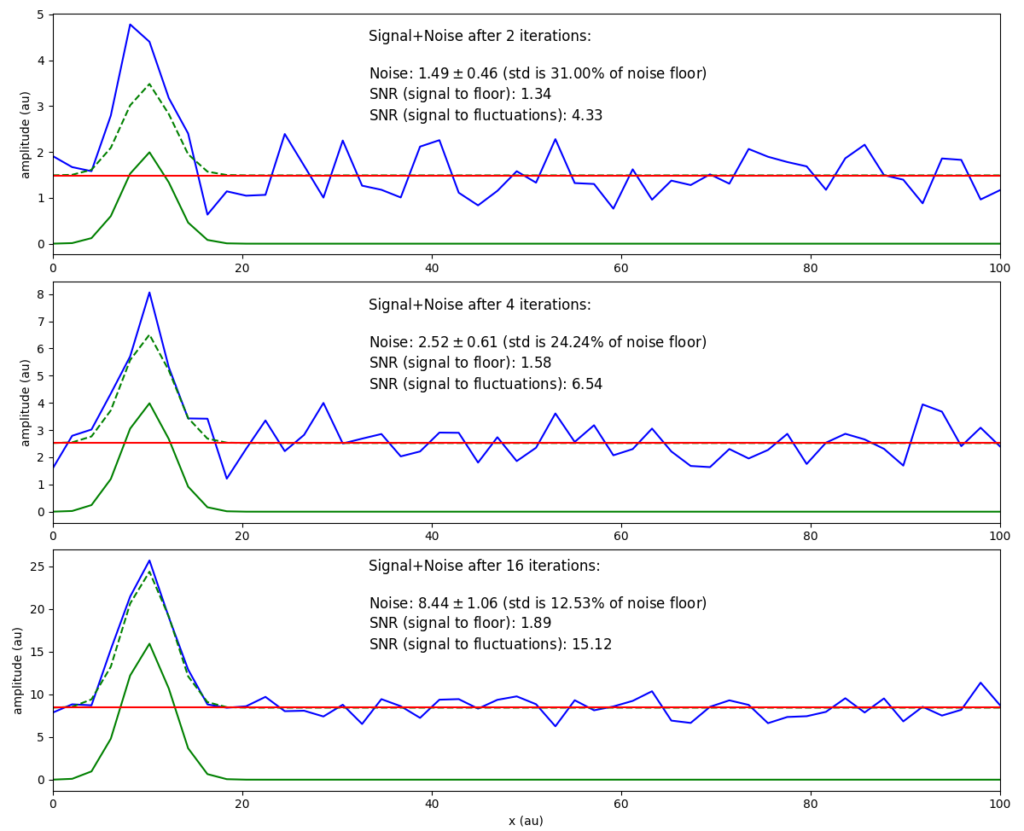
By repeating a measurement $n$ times, the signal content starts to dominate the noise. In the following plots, I show the summed up detected signal in blue. This detected signal contains signal and noise. To make the underlying components visible, I highlight the signal portion in green (solid line: pure signal, dashed: pure signal with noise floor offset). The red line signifies the noise floor.

Definition and different approaches

In the plot above I’ve skipped a few explanations in order to get a visual aid showing the core idea of this post: noise fluctuations tend to flatten out compared to signal contributions.

Yet, I need to get back onto some definitions. Namely, in the plots above, I have worked with two different signal-to-noise (SNR) definitions: signal to floor, and signal to fluctuations.

I reuse the idea stated in the other post that a measurement $M_j$ accumulates the detected $D_j$ signal $S_j$ and noise $N_j$ contributions:
$$M_n = \sum\limits_{j=0}^n D_j = \sum\limits_{j=0}^n (S_j + N_j)$$

In either of the definitions of signal to floor or signal to fluctuations the signal adds up with each measurement. Hence, the average signal $S_\mathrm{avg}$, added at every iteration, is also S ($S_\mathrm{avg}=\frac{nS}{n}=S$). In our case, we chose the amplitude $S=1.$ For the noise on the other hand, we have assumed a uniformly distributed function for values between $[0,1]$ (with $N=1$ the chosen noise amplitude). The mean value of such a distribution is $N_\mathrm{avg}=\frac{N}{2}$.

Hence, with these numerical values, the signal to floor converges to
$$
SNR_\mathrm{floor} = \frac{S_\mathrm{avg}}{N_\mathrm{avg}} = \frac{S}{N/2}|_\mathrm{S=N=1} = 2.
$$

Put differently, the SNR in this definition converges to value $Q=2k$ if the amplitude of the signal is fraction $k$ of the amplitude of the noise:
$$
\begin{split}
\frac{S}{N} &= k \\
\Rightarrow\quad SNR &= \frac{kN}{N/2} = 2k.
\end{split}
$$

This definition and scaling behavior is good and well, but I feel unsatisfied with the numerical result. It doesn’t convey the fundamental idea of how much the signal is overpowering the … noise(?). Intuitively, when talking about “noise”, I actually mean the fluctuations. And the signal-to-noise ratio should tell me how easy it is to discern a signal peak among the random noise peaks. The amplitude of the noise peaks (the difference between random highs and lows) diminishes as we add up the noise contributions of more and more measurements.

This understanding is what I denote as signal to fluctuations: as the alternative SNR value
$$
SNR_\mathrm{fluct} = \frac{S}{\Delta N},
$$
with $\Delta N = \sigma(N) = \sqrt{\mathrm{V}[N]}$.

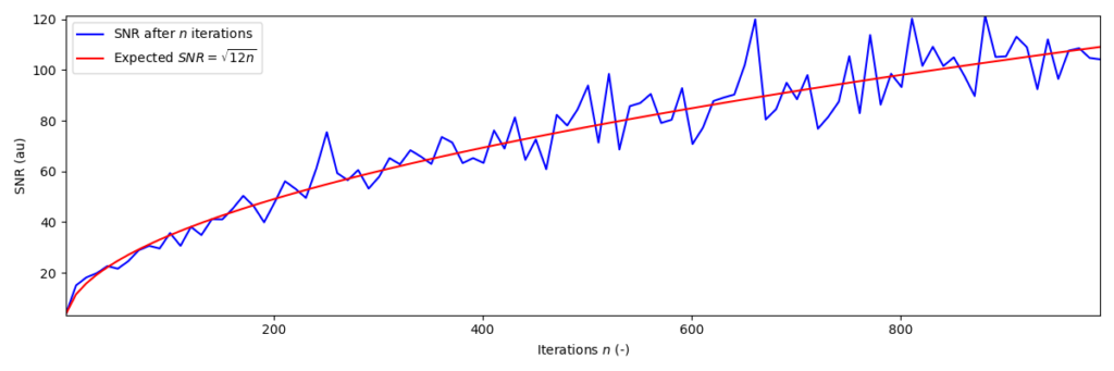
This also corresponds to the heuristically derived SNR expression, for I have additionally shown that it scales with the square root of the $n$ conducted measurements:

$$SNR = \sqrt{n}\frac{S}{\sigma_N}.$$

The standard deviation $\sigma$ of uniformly distributed noise is $\sigma = \sqrt{\mathrm{V}[x]} = \sqrt{\frac{1}{12}(b-a)}$, with $a=0$, $b=1$ the values of the distribution in the present case. All put together we once again find the square root scaling of the SNR

$$SNR = \sqrt{n}\frac{S|_{S=1}}{\sigma_N} = \sqrt{n}\frac{1}{\sqrt{1/12}} = \sqrt{12n}.$$